Laplace-Hamming Filter Example

By: Michael T. Kuczynski, 2025
License: CC-BY
How to cite: Cite the ORMIR_XCT publication: Kuczynski et al., (2024). ORMIR_XCT: A Python package for high resolution peripheral quantitative computed tomography image processing. Journal of Open Source Software, 9(97), 6084, Kuczynski et al. (2024)

Aims¶

This Jupyter Notebook provides an example of running the Laplace-Hamming segmentation from the ORMIR_XCT package.
First, a Laplace-Hamming filter is applied to the image to smooth and enhance edges.
Then, a global threshold is applied to segment the image.
The input parameters to the Laplace-Hamming filter and segmentation are selected based on the paper by Sadoughi, et al. JBMR. 2023. Sadoughi et al. (2023). Specifically,
- Laplace epsilon = 0.45
- Laplace cut off frequency = 0.3
- Hamming amplitude = 1.0
- Lower threshold = 475 per mille
Table of contents
Step 1: Imports
Step 2: Laplace-Hamming Filter
Step 3: Global Threshold
Step 4: Compare to seg_gauss

Step 1: Imports:¶

Import modules/packages and set the input image path.

import os
import numpy as np
import SimpleITK as sitk
import matplotlib.pyplot as plt

from ormir_xct.core.segmentation.seg_gauss import seg_gauss
from ormir_xct.core.segmentation.fft_laplace_hamming import fft_laplace_hamming

Step 2: Laplace-Hamming Filter:¶

Read in an image and run the Laplace-Hamming filter. Then, compare the filtered image to the original.

# Read in an image
joint_seg_path = os.path.join("images", "GRAY_JOINT.nii")
output_path = "images"

gray_img = sitk.ReadImage(joint_seg_path, sitk.sitkFloat32)
gray_img_np = sitk.GetArrayFromImage(gray_img)

# Run the Laplace-Hamming filter
lh_image_np = fft_laplace_hamming(gray_img_np, laplace_epsilon=0.45, lp_cut_off_freq=0.3, hamming_amp=1.0)

slice_index = lh_image_np.shape[0] // 2

plt.figure(figsize=(12, 6))

# Plot the original image slice
plt.subplot(1, 2, 1)
plt.imshow(gray_img_np[slice_index, :, :], cmap="gray")
plt.title("Original Image (Middle Slice)")
plt.axis("off")

# Plot the filtered image slice
plt.subplot(1, 2, 2)
plt.imshow(lh_image_np[slice_index, :, :], cmap="gray")
plt.title("Laplace-Hamming Filtered Image (Middle Slice)")
plt.axis("off")

plt.tight_layout()
plt.show()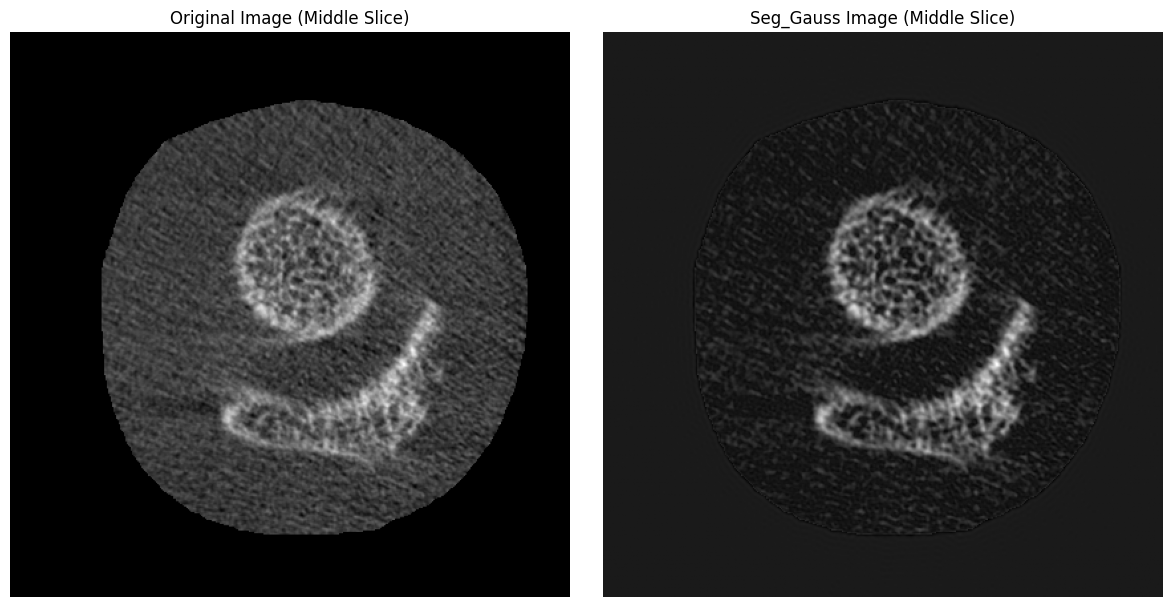

Step 3: Global Threshold:¶

Next, apply a global threshold of 475 per mille to the Laplace-Hamming filtered image. A Threshold of 475 per mille is 0.475 * the maximum intensity value of the image in native units. Since we are using a HR-pQCT (AIM) image that was converted to NIFTI using the ITKIOScanco module, our image is in HU. Assuming mu_scaling = 8192, mu_water = 0.2396, we can convert our image to per mille as follows:

Get the maximum intensity of the image in HU ( $max_{HU}$ )
$\mu = \frac{\text{max}_{HU} \cdot \mu_w}{1000} + \mu_w$
(1)

\text{native} = \mu \times 8192

(2)

\text{threshold} = \text{native} \times 0.475

(3)

\text{threshold}_{HU} = 1000 \times \frac{\left(\frac{\text{threshold}}{8192} - \mu_w\right)}{\mu_w}

(4)

Since the maximum of our test image is 3,828, our threshold is 1,293.3 HU.

lh_image = sitk.GetImageFromArray(lh_image_np)
lh_image.CopyInformation(gray_img)

lh_seg = sitk.BinaryThreshold(lh_image, 1293, 10000, 1, 0)
lh_seg_np = sitk.GetArrayFromImage(lh_seg)

Step 4: Compare to seg_gauss:¶

Compare the Laplace-Hamming segmentation to the seg_gauss function.

ipl_mask = seg_gauss(gray_img, 1170, 10000, value_in_range=1, value_outside_range=0, 
                     sigma=0.8, support=1, use_image_spacing=False)
ipl_mask_np = sitk.GetArrayFromImage(ipl_mask)

slice_index = (gray_img_np.shape[0] // 2)-25

plt.figure(figsize=(6, 6))

# Plot the original image slice
plt.subplot(2, 2, 1)
plt.imshow(gray_img_np[slice_index, :, :], cmap="gray")
plt.title("Original Image")
plt.axis("off")

# Plot the seg_gauss image
plt.subplot(2, 2, 2)
plt.imshow(lh_image_np[slice_index, :, :], cmap="gray")
plt.title("Lp_Hamming Filtered Image")
plt.axis("off")

# Plot the filtered image slice
plt.subplot(2, 2, 3)
plt.imshow(ipl_mask_np[slice_index, :, :], cmap="gray")
plt.title("Seg_gauss Segmentation")
plt.axis("off")

# Plot the seg of lp_hamming
plt.subplot(2, 2, 4)
plt.imshow(lh_seg_np[slice_index, :, :], cmap="gray")
plt.title("Lp_Hamming Segmentation")
plt.axis("off")

plt.tight_layout()
plt.show()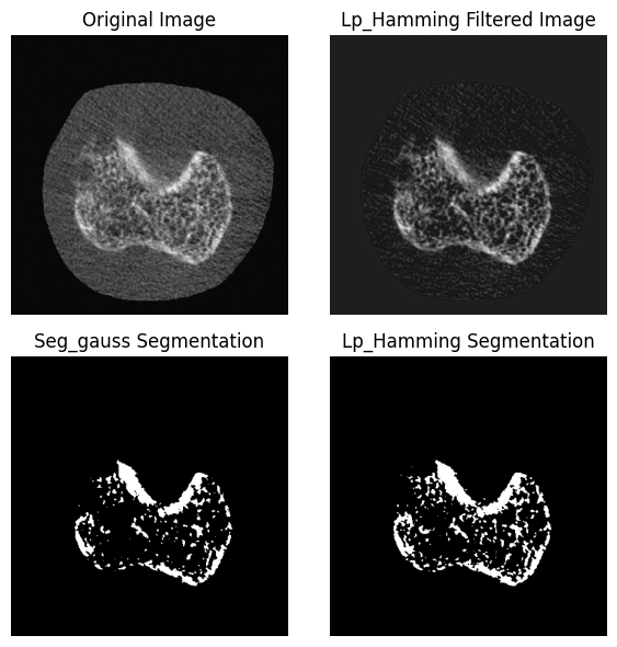

Notebook created using the template of the ORMIR community (version 1.0, 2023)

References¶

Kuczynski, M. T., Neeteson, N. J., Stok, K. S., Burghardt, A. J., Hernandez, M. A. E., Vicory, J., Tse, J. J., Durongbhan, P., Bonaretti, S., Wong, A. K. O., Boyd, S. K., & Manske, S. L. (2024). ORMIR_XCT: A Python package for high resolution peripheral quantitative computed tomography image processing. Journal of Open Source Software, 9(97), 6084. 10.21105/joss.06084
Sadoughi, S., Subramanian, A., Ramil, G., Burghardt, A. J., & Kazakia, G. J. (2023). A <scp>Laplace–Hamming</scp> Binarization Approach for <scp>Second‐Generation HR‐pQCT</scp> Rescues Fine Feature Segmentation. Journal of Bone and Mineral Research, 38(7), 1006–1014. 10.1002/jbmr.4819